Repository navigation
Technical Concepts
ℹ️ NOTICE : The normative version of this reference is in the source tree.
This file contains an attempt to rerender this information using Github's Markdown variant.
The result is somewhat flawed, and probably won't work at all for users using dark mode because of difficulties rendering math.
This document explains the theoretical background for the PyWeight application. Ordinary users are not expected to need to read this.
Users who wish to read a light overview of the ideas here and a discussion of weight loss using PyWeight may find the essay by PyWeight's primary author informative.
PyWeight is intended to make weight management easier by solving two problems:
-
Fluctuations in body weight tend to swamp real changes on a daily basis, making it difficult to track progress
-
Determining a meal plan on the basis of calories in - calories out (CICO) is difficult, because determining your total daily energy expenditure (TDEE) is hard, and accurately counting every calorie you eat is arguably even harder.
The method employed by PyWeight involves estimating the rate of weight loss (in kg/day) by taking the derivative of statistically smoothed daily measurements. This basic idea was originally suggested by The Hacker's Diet, though PyWeight contains a number of improvements.
For a given period of d days, if the weight loss goal was g kilograms and the actual weight loss was w kilograms, then the difference between the goal and the actual change is (g - w) / d, in kilograms per day.
This approach not only gets rid of most fluctuations (by taking the derivative of a smoothed value), it also determines the degree of success and failure independently of any knowledge about meal planning. It simply answers the question "did the user lose too much weight, or not enough?".
However, telling the user "try to lose 0.01 more kilograms every day" is not useful advice. Regardless of whether or not the user is precisely planning meals, "try to eat 75 fewer calories every day" is far more actionable, because it translates in a straightforward way to actual meal-time decisions.
Therefore, PyWeight needs to estimate how many calories are associated with a given quantity of weight loss. If we can calculate the size of the calorie deficit required to lose g kilograms, and the size of the deficit required to lose w kilograms, then we can trivially calculate the number of calories the user missed their target by over the d day period, and therefore how many calories they missed their target by on a daily basis.
The constraint this program works under is that this calculation has to be made without reference to meal plans or knowledge of the user's TDEE. The rest of this document details how to do that.
Changes in weight are the result of a deficit or surplus in energy intake to energy expended by the body. The body releases energy for use in its activities by breaking down the chemical bonds in several molecules. These molecules can either come from food and substances like glycogen created by the body from food, or they can come from energy stored in the body, mostly as fatty acids.
If we assume a constant energy expenditure, then a long term reduction in daily food intake of 100 calories will mean that the body will have to take that 100 calories from its energy storage. The byproducts of the body's energy creation process, largely carbon dioxide and water, will be expelled into the environment, reducing the amount of mass the body permanently stores.
This suggests a straightforward way of determining the size of the deficit required to lose a kilogram of mass. If an individual eats n fewer calories than their body consumes over a period of time, those n calories will necessarily (by conservation of energy) be taken from its energy stores instead. If these energy stores are in the form of fat tissue, we can determine the expected amount of weight loss associated with the deficit using the typical energy density of fat tissue. No information about the individual or their diet is required.
Because of the obvious usefulness of such a simplification, it is unsurprising that the claim that a pound of fat contains 3500 calories has become a piece of common "knowledge". If this is true, then any person who wants to lose 50 pounds needs to achieve a total deficit of 175,000 calories. They will therefore lose this 50 pounds via any method of achieving this deficit, whether it takes weeks, months, or years.
Unfortunately, this commonly held belief is wrong: a pound of fat contains about 4280 calories (just over 9400 calories per kilogram).1 Obviously, fixing the incorrect value would not be too difficult, but the apparent straightforwardness of this approach masks two crucial assumptions:
-
The individual attempting to lose weight will have a constant energy expenditure over the course of the diet.
-
The weight lost over the course of the diet will be entirely from the fat the body uses for energy.
Both of these assumptions are incorrect, and so we need to think about the implications for the determination of caloric deficits and dietary strategy.
It is easy to see that the assumption of a constant energy requirement is incorrect. A person who weighs 150 kilograms will need more energy than one who weighs 100 kilograms, simply in virtue of needing to expend more energy to move the extra 50 kilograms from point A to point B, and because those 50 kilograms contain cells which need energy to sustain themselves. Published equations for basal metabolic response, and therefore also for TDEE, rely on body weight, height, and other characteristics. Since one's weight changes over the course of a diet, one's energy requirements will also.
For some common estimates of basal metabolic response, such as the Mifflin - St. Jeor equation, energy needs are linear with body weight. If true, this is convenient because it suggests that one's weight over time follows a simple first order differential equation.
Assuming the Mifflin - St. Jeor equation accurately describes the behavior of metabolism, weight over time is:
where b is the constant
Here, intake is the daily calories consumed, activity is a multiplier indicating the level of activity relative to the BMR (e.g. 1.4 indicates a fairly inactive adult), and sex is 0 for women and 1 for men. Units are calories, centimeters, and years. Note that the 7700 value reflects the expected energy density of weight loss: the assumption made here is the metric equivalent of 3500 calories per pound.
Solving this equation suggests that someone who eats like a metabolically identical person with their goal weight will exponentially approach that weight.
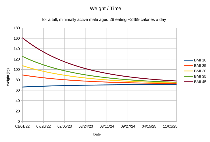
Unfortunately, while it makes for a nice graph, the assumption that the energy expenditure of dieters varies linearly with their current weight is also false, according to research.
Rather, metabolism has two transitory effects, one immediate and the other long lasting. Both resist changes in weight, whether increases or decreases.
When someone begins eating at a calorie deficit, the body responds by reducing the amount of energy it consumes. (Despite the way this happens in the popular imagination, the effect is not magical. Their body is simply doing less work than it did before. Someone eating at a deficit is likely to be more tired than normal, feel less like exercising, and some of their body's regular processes may be disrupted.) Thus, even if published equations accurately estimate an individual's TDEE, the estimate will (temporarily) become inaccurate while they are trying to lose weight.
Similarly, the body may behave as though it remembered its previous weight (lower or higher) and was trying to get back to that. The NIDDK model of diet performance suggests that someone who is 235 lbs, having recently gained 85 pounds will consume about 400 more calories per day than an otherwise metabolically equivalent individual of the same weight who recently lost 85 pounds.2 3
This effect is partially explained by differences in body composition. Lean body mass requires more energy to maintain than does fat. But there may also be some active component, whereby the body reduces its metabolic rate following weight loss more than can be explained by changes in body composition.
The existence of this effect — at all — is contentious. Some studies found no such effect.4
We suggest that while such an effect may make sense both physiologically and in terms of selective pressure, it is likely to be temporary. The NIDDK model shows a much larger effect for gaining weight than it does for losing weight. There is only a 50 calorie a day difference in that model between the 235 pound person mentioned above who lost 85 pounds and someone who has maintained at 235 pounds for years, while the person who gained 85 pounds burns 350 calories a day more. But few 235 pound people have weighed that much their entire adult lives: you only become someone who maintains at 235 pounds by previously weighing much less and gaining weight. In other words, transitioning between these profiles must be possible, though it may take more time than the typical study length of the research used in developing this model.
PyWeight takes a very interesting approach to these complexities, which also happens to be the simplest one: we completely ignore them.
If our approach involved trying to determine the user's TDEE in order to provide them with a recommended number of calories to consume, we would have to take all this into account. However, we don't do this. The PyWeight approach is to determine the difference between the user's caloric target and their intake. Metabolism obviously has a direct effect on the number of calories required to maintain one's weight, but it has an almost negligible effect on the energy density of given unit of weight loss.
Above, we discussed the naive claims that body composition changes are entirely in the amount of fat retained, and that this fat has an energy density of 3500 calories.
As it turns out, while both of these claims in incorrect, their effects point in opposite directions and therefore 3500 calories / pound is a more reasonable estimate than expected. As it turns out, the lean body mass lost during weight reduction has a typical density of about 824 calories a pound1, and therefore the 3500 calorie per pound estimate is almost exactly right if about 75% of the weight you lose is from fat.
That said, such an estimate clearly can't be right in many cases. If we imagine someone slightly underweight continuing to lose weight, they will at some point have no more fat to lose, and will therefore lose lean mass instead. We should expect the fraction of weight loss due to fat to be a continuous function, approaching 0 for individuals for very little fat mass, and approaching some high fraction (though not 1) for individuals with a large amount of fat losing a comparatively small amount of weight.
Hall5 and Hall et. al6 provide a model describing the behavior of this ratio, and it is this model on which PyWeight's calculation of weight loss composition is based.
The Hall paper takes an equation from Forbes7:
Looking at this equation, we can see that it suggests a static relationship between fat mass F and lean mass L. An individual described by this equation with only one kilogram of fat would have 14.2 kilograms of fat free mass. Such an equation clearly could not describe everyone. Forbes' equation was an empirical fit to a number of physically similar women.
Hall effectively conjectures that this relationship extends to other body types as well, satisfying the equation
for a constant A specific to each body type.
If we let Li, Lf, and Fi, Ff describe the body's lean and fat masses before and after weight loss (respectively), then since by definition Lf = Li + ΔL,
and the A on each side of the equation conveniently drops out. At first glance this equation doesn't seem to have simplified things, but notice that ΔL is just the portion of total change in mass not attributable to change in fat mass:
We make that substitution and isolate Ff.
Making the substitution Ff = 10.4 u,
For positive u, equations of the form u exp(u) = v have the unique solution u = W(v), where W is the Lambert W function. Back-substituting,
Hall et. al looked at studies of weight loss and found that this equation does accurately describe relative changes in fat and lean mass in a wide variety of body types.
We know that Fi = BFPi · Mi where BFPi designates the initial body fat percentage. This is something we can estimate on the basis of other variables (see below) or rely on the user to input directly. The initial body weight is obviously available as we have the data that the user entered in the PyWeight log. Determining changes in body weight is of course one of the main functions of PyWeight — so putting all of this together, we can easily estimate the fraction of a user's weight loss which is due to fat loss.
The caloric deficit associated with that weight loss is therefore simply the sum of the loss associated with each source weighted according to its calorie density:
So we can calculate, for a given weight change w over a period of d days, the size of the daily caloric deficit associated with that change. Since we can calculate the same value for the desired weight change over the same period, we can easily determine the difference between the goal and what was achieved and present this to the user!
The authors do not know of any other weight management tool that takes the same approach to estimating body composition changes over time. The NIDDK model and its associated online tool do allow planning weight loss over time, but the approach to dieting that this tool takes is (in the opinion of the PyWeight authors) flawed.
The NIDDK model assumes that weight changes will be achieved via a constant intake of whatever number of calories is appropriate to hit the goal weight by some date.
For large changes in weight, the results are often unreasonable. The web application recommends that a 23 year old, 5 foot 11 inch male with a starting weight of 200 pounds who wants to lose a fairly reasonable 40 pounds in 180 days should cut his calorie consumption by over 1000 calories a day at the outset. This is large enough to be difficult to maintain, and in some cases the program can be made to output values that are clearly unsafe.
Even though PyWeight is based on the same research as the NIDDK model, the advice it provides is far more reasonable. The PyWeight approach to weight loss targets a constant rate of weight loss, rather than a constant caloric intake. The result is far more consistent with weight loss guidelines given by public health organizations. Here is what the same person's experience would be in PyWeight:
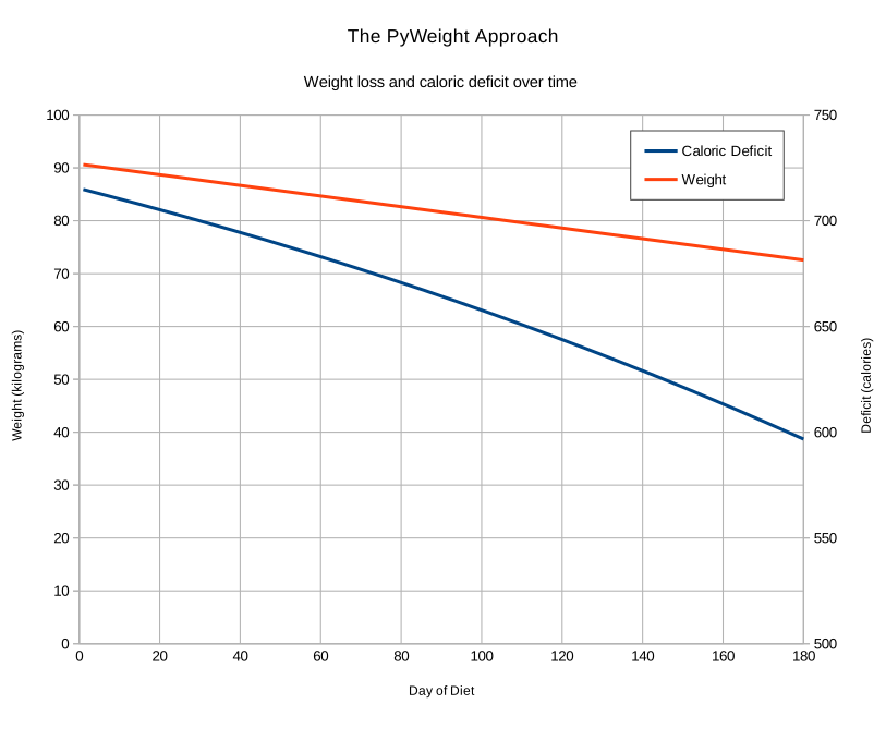
The difference is remarkable. With PyWeight, the same individual would start at a deficit of only 715 calories a day, which would drop to just under 600 by the end of the diet. This feels realistically achievable. (Note that because the user's daily energy expenditure would drop over the course of the diet, the end would not necessarily be easier than the beginning, despite a smaller deficit being required.)
PyWeight's primary author lost about 30 pounds with versions of the program (some built with spreadsheets) that assumed the naive 3500 calorie per pound density of weight change. PyWeight's approach of only considering differences between desired and achieved weight changes tends to smooth away mistakes like this, because in practice the advice usually amounts to "eat a little more the next two weeks", or vice versa.
The impetus for fixing this is in part just technical accuracy, but also because it's important to not create in the user an unreasonable sense of how many calories their food contains. If the user attempts to follow the program's advice, and doesn't achieve the expected results, they are likely to revise their future behavior. This is good in the sense that they will still hone in on their desired outcome, but bad in the sense that they will end up thinking a 300 calorie change is larger, or smaller, than it really is.
Hall et. al6 think the 3500 calorie / pound estimate is quite bad. They write,
The recommendation that an overweight or obese person should expend an additional daily 100 kcal (420 kJ) in walking (ie, walking one mile a day), given the new rule of thumb discussed above, would result in a weight loss of ∼ 10 lb (4.5 kg) over 5 y, as opposed to a loss of 50 lb (23 kg) if the 3500 kcal per pound rule is used.
Does the 3500 calorie / pound rule actually indicate a loss of 50 pounds over 5 years? In our judgment, it does not. The authors are imagining a hopelessly naive use of the rule that assumes that each individual's TDEE remains constant over time, despite weight loss. In other words, this version of the rule holds that walking one mile a day more than you currently do will eventually kill you from starvation unless you eat to compensate.
Certainly you can find examples of the rule being applied in ways as naive as this, but there's no reason to treat this as an inherent flaw of the simple rule of thumb. Rather, given the assumption that an individual's TDEE is linearly related to their current weight, the 3500 calorie rule actually generates the rather beautiful differential equation and graph shown above — where the number of calories you eat results in approaching an equilibrium weight. It's still wrong, but not as dangerously so as Hall et. al imagine.
Recall from the previous section that PyWeight determines the energy density of weight loss from three variables: initial body weight, change in body weight, and initial body fat percentage. The first two are trivially known to the program because of how it operates. The latter is more complicated. PyWeight can (and does) allow the user to enter this value manually, but most users will not know it with any accuracy.
The PyWeight authors have reviewed a number of models for estimating body fat percentage using a variety of other variables. All of them have flaws. Some haven't been tested; others have been tested but have been found to be inaccurate.
One of the more promising methods is by Lee et al.8 A number of issues has resulted in our ruling it out at present. The model is linear equation of a number of variables, but most of the other promising models show some non-linear effects. On the positive side, it does look at race as an explicit factor, but because it ended up as a significant variable in the model, PyWeight would have to request this data from the user. PyWeight would also have to exclude all races other than the few considered by the model, and it is not obvious how to do this in a reasonable way. Some other potential issues are addressed in comments in the source file.
At present PyWeight uses the CUN-BAE equation9. This approach is limited in that all the subjects in the study were white Americans, but this does have the benefit that race isn't an explicit variable in the model (which is at present unworkable for the reasons given above). This model has the strong benefit that it has been subjected to external validation by Cui et. al10 and found to be quite accurate, including surprisingly so for non-White Americans.
This model is a quadratic equation in weight, age, height, and sex. An explicit reference to sex is a complication, but a required one, because women typically have body fat percentages significantly higher than do men.
One unfortunate limitation noted in our literature review is that no studies we found looked at estimations of body fat percentage in transgender, non-binary, or intersex people.
A simplistic approach, but clearly an improvement on nothing at all, is to allow the user to select their position on a spectrum from male to female. It is not wholly unreasonable to expect that a PyWeight user on hormone replacement therapy might expect to have body fat somewhere in between that typical of cisgender male and female human bodies. At present, then, PyWeight makes this choice available to users as a simple slider.
One of the more significant practical difficulties of weight management is the complexity of progress tracking. A typical person's weight fluctuates by multiple pounds over the course of a single day, meaning that weight measured on a daily basis will vary strongly depending on exactly when the weight is measured and the amount of eating and drinking in the previous 24 hours.
Because PyWeight is based on the principle of fine-tuned adjustments to intake, it has a strong need for an accurate measurement of weight change over time.
Rather than looking at day to day variations, which are almost impossible to measure with any accuracy, PyWeight estimates and provides feedback on weight changes over a longer period of time — 2 weeks by default.
Asking PyWeight users to weigh themselves every two weeks would have many of the same flaws as daily measurements because these individual point estimates would themselves be imprecise. Rather, PyWeight asks users to weigh themselves on a daily basis and computes a regression line through the resulting data. The derivative of this line (in this case, the slope) is the average rate of weight loss over the period.
One straightforward way of working with the data would be to generate a new linear regression for each new period of weight loss. This has an obvious flaw: each period's estimated weight loss would be based on only data from that period, and so the estimated starting weight and ending weight for the period would frequently not align with the estimates used for the previous and subsequent period. In addition to the issue of throwing away valuable data, this also risks introducing bias: if the user's behavior changes on a consistent bi-weekly basis, the starting point of each period could end up higher than the ending point of the previous one, resulting in a consistent over-estimate of the amount of weight lost.
Rather, PyWeight takes a more sophisticated approach. We fit a spline to the user's entire weight history. Specifically, we choose a linear spline with knots at each of the period endpoints, and fitting done with least squares. This mirrors the behavior of a linear regression, but adds the additional constraint that the resulting fit must be continuous.
A fit of this type means that the data must be re-interpolated whenever a point is added or edited, but on any modern hardware these fits are fast enough for this to be a negligible concern.
One possible alternative is a moving average. For some types of weight loss program this approach would be appropriate, but as outlined above, the PyWeight approach is to have the user focus on a constant rate of weight loss, with periods of consistent intake punctuated by minor adjustments. A moving average would fluctuate too much and be too dependent on data recency to give good results for PyWeight.
The resulting spline fit is used to generate many of the data points needed by PyWeight equations. For example, rather than use the user's first weight entry as the initial weight for the estimate of weight change density, PyWeight uses the first point on the spline instead. Likewise, for the user's current weight, rather than use the latest entry, the last point on the spline is used.
The use of a spline also makes the calculation of the weight loss density for a given period straightforward. Because in the Hall model the density of a given amount of weight loss depends on the initial body weight, not the wait at the start of any arbitrary period, we determine the caloric deficit associated with all weight change from the first day to the beginning of the most recent period, and the deficit associated with the weight change from the first day to the present. Subtracting the former from the latter yields the portion of the total caloric deficit associated purely with the current period.
An exactly parallel method is followed to derive the caloric deficit associated with the desired weight loss for the current period. Determining the daily number of calories the user should consider adding or removing from their intake is thereby made simple.
1 Hall, K D. “What is the required energy deficit per unit weight loss?.” International journal of obesity (2005) vol. 32,3 (2008): 573-6. doi:10.1038/sj.ijo.0803720 ↩️
2 The Body Weight Planner by the National Institute of Diabetes and Digestive and Kidney Diseases: https://www.niddk.nih.gov/bwp ↩️
3 https://adamfontenot.com/post/statistics-assisted_weight_loss_with_pyweight ↩️
4 Weinsier, R L et al. “Do adaptive changes in metabolic rate favor weight regain in weight-reduced individuals? An examination of the set-point theory.” The American journal of clinical nutrition vol. 72,5 (2000): 1088-94. doi:10.1093/ajcn/72.5.1088 ↩️
5 Hall, Kevin D. “Body fat and fat-free mass inter-relationships: Forbes's theory revisited.” The British journal of nutrition vol. 97,6 (2007): 1059-63. doi:10.1017/S0007114507691946 ↩️
6 Hall, Kevin D et al. “Quantification of the effect of energy imbalance on bodyweight.” Lancet (London, England) vol. 378,9793 (2011): 826-37. doi:10.1016/S0140-6736(11)60812-X ↩️
7 Forbes, G B. “Lean body mass-body fat interrelationships in humans.” Nutrition reviews vol. 45,8 (1987): 225-31. doi:10.1111/j.1753-4887.1987.tb02684.x ↩️
8 Lee, Dong Hoon et al. “Development and validation of anthropometric prediction equations for lean body mass, fat mass and percent fat in adults using the National Health and Nutrition Examination Survey (NHANES) 1999-2006.” The British journal of nutrition vol. 118,10 (2017): 858-866. ↩️
9 Gómez-Ambrosi, Javier et al. “Clinical usefulness of a new equation for estimating body fat.” Diabetes care vol. 35,2 (2012): 383-8. doi:10.2337/dc11-1334 ↩️
10 Cui, Zhaohui et al. “Evaluation of anthropometric equations to assess body fat in adults: NHANES 1999-2004.” Medicine and science in sports and exercise vol. 46,6 (2014): 1147-58. doi:10.1249/MSS.0000000000000213 ↩️